Analytic Hierarchy Process

One Thursday morning, Charles, instead of attending his Management Science Techniques for Consultants class, was mulling over his four job offers. His offers came from Acme Manufacturing, Bankers Bank, Creative Consulting, and Dynamic Decision Making. He knew that factors such as location, salary, amount of management science (which he loved), and long term prospects were important to him, but he wanted some way to formalize the relative importance, and some way to evaluate each job offer. Luckily, he attended the following Tuesday class of MSTC, who showed him one way to think about these problems. This technique is called the Analytic Hierarchy Process.

The first step in AHP is to ignore the jobs and just decide the relative importance of the objectives. Charles does this by comparing each pair of objectives and ranking them on the following scale: Comparing objective i and objective j (where i is assumed to be at least as important as j), give a value  as follows:

Table 1: Pairwise comparison values

Of course, we set  . Furthermore, if we set  , then we set  . Charles, thinking hard about his preferences, comes up with the following table:

Table 2: Preferences on Objectives

Now, the AHP is going to make some simple calculations to determine the overall weight that Charles is assigning to each objective: this weight will be between 0 and 1, and the total weights will add up to 1. We do that by taking each entry and dividing by the sum of the column it appears in. For instance the (Location,Location) entry would end up as  . The other entries become:

Table 3: Weights on Objectives

This suggests that about half of my objective weight is on salary, 30% on amount of management science, 13% on long term prospects, and 9% on location.

Now, why does this magical transformation make sense? If we read down the first column in the original matrix, we have the values of each of the objectives, normalized by setting the value of location to be 1. Similarly, the second column are the values, normalizing with salary equals 1. For a perfectly consistent decision maker, each column should be identical, except for the normalization. By dividing by the total in each column, therefore, we would expect identical columns, with each entry giving the relative weight of the row's objective. By averaging across each row, we correct for any small inconsistencies in the decision making process.

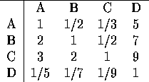
Our next step is to evaluate all the jobs on each objective. For instance, if we take Location, if we prefer to be in the northeast (and preferably Boston), and the jobs are located in Pittsburgh, New York, Boston, and San Francisco respectively, then we might get the following matrix:

Table 4: Location Scores

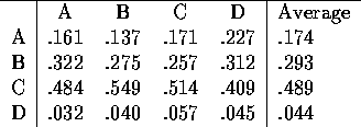
Again we can normalize (divide by the sums of the columns, and average across rows to get the relative weights of each job with regards to location. In this case, we get the following:

Table 5: Relative Location Scores

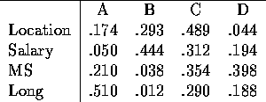
In words, of the the total ``Location Value'' available, Job C and about 50%, B has about 30%, A has about 17% and D has about 4%. We can go through a similar process with Salary, amount of MS, and long term prospects. Suppose the relative values for the objectives can be given as follows:

Table 6: Relative scores for each objective

Recalling our overall weights, we can now get a value for each job. The value for Acme Manufacturing is

Similarly, the value Bankers Bank is

The value for Creative Consultants is .335, and that for Dynamic Decision is .238. Creative Consultants it is! Charles immediately makes his decision in order to have extra time to study for the MSTC exam.

The Analytic Hierarchy Process is a method for formalizing decision making where there are a limited number of choices but each has a number of attributes and it is difficult to formalize some of those attributes. Note in this example, we did not collect any data (like miles from a preferred point or salary numbers). Instead, we use phrases like ``much more important than'' to extract the decision makers preferences.

The AHP has been used in a large number of applications to provide some structure on a decision making process. Note that the system is somewhat ad-hoc (why 1-9 range?) and there are a number of ``hidden assumptions'' (if i is weakly preferred to j and j weakly preferred to k, then a consistent decision maker must have i absolutely preferred to k, which is not what my idea of the words means). Furthermore, an unscrupulous can easily manipulate the rankings to get a preferred outcome (by using a non-management science technique called ``lying'') Despite the rather arbitrary aspects of the procedure, however, it can provide useful insight into the tradeoffs embedded in a decision making problem.